It’s hard to imagine today’s world without Microsoft Excel. This program helps many people, regardless of their occupation. It’s needed both for some important projects for work and for ordinary planning.

However, despite the fact that it’s so popular and necessary, it has many functions that most users can’t figure out on their own. For example with the SUBSTITUTE function. It’s really not that complicated, but you should still look at the detailed instructions to make it easier in the future.

What to do to use the SUBSTITUTE function in Microsoft Excel

Microsoft Excel users will agree that this program is very handy and functional. However, many people won’t be able to intuitively understand how to use it. This program has a lot of rules and you need to know a lot of formulas. Even so, it’s not too scary. It’s possible and even quick to figure out, you just need to know what algorithm you want the formula to work and do all that is required of it.

The main purpose of this function is to return a text string where the old text has been replaced by new text. There’re some small rules that you should know before you start working with this function. Remember that this formula is case-sensitive. It’s also best to use this function when you want to change some specific text to another text.

Be careful not to use a negative number as an argument, or the system will generate an error. To get started with this function, you’ll need to familiarize yourself with its arguments. This will allow you to use the SUBSTITUTE function right away.

What arguments of the SUBSTITUTE function do need to know in order to use it

In fact, the arguments of the SUBSTITUTE function are only 4. They’re easy to remember and use as you work through Microsoft Excel. To work with this function, you’ll need:

• text – the source string used to perform the replacement.
• old_text – old text where the replacement will take place
• new_text – the new text which will be replaced
• [instance_num] – determines which occurrence of the text will be replaced. If the argument isn’t specified, the entire text will be replaced.

What steps to take to use the SUBSTITUTE function in Microsoft Excel

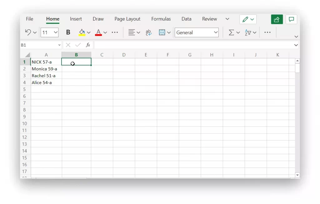
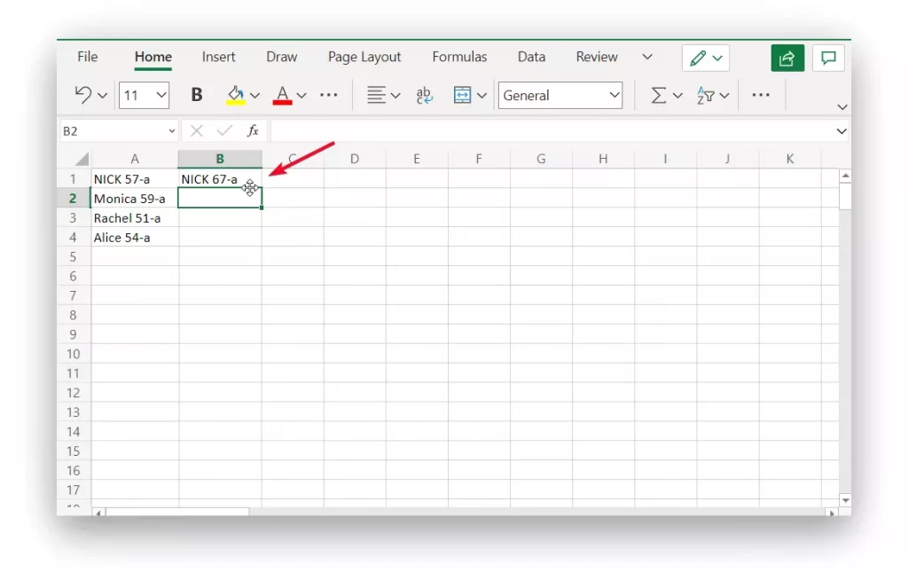
The SUBSTITUTE function can help you replace all instances of a particular text with new text. If in the conditional table, in cell A1 you need to replace the serial number of participant. From having [ name number – a ], for example NICK 57-a, replace it with NICK 67-a. The reason for this may be that in any company, training center and others may change groups. Accordingly, this change should be made to all existing tables. If your goal is to replace all instances of text with another using the SUBSTITUTE function in Microsoft Excel, you need to follow these steps:

• To replace all instances of text with another using the SUBSTITUTE function, you need to start Microsoft Excel.
• Next, fill in your data in the table or open an existing one to make changes.

• First, you need to select the cell to display the result.

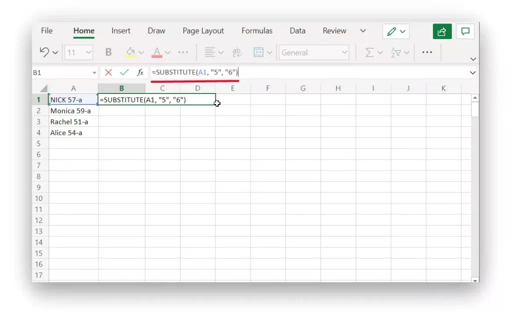
• Next you need to enter in the line for the function ‘=SUBSTITUTE(A1, “5”, “6”)‘. This function means that from cell A1 the digit 5 will be replaced by 6. In your case, you can specify another cell or text to replace it.

• Once you’ve added the function text, you need to click on the ‘Enter’ button for it to apply.

However, it’s worth remembering that this function can be extended. It can’t only change a single digit. You can specify any text. This is where you could replace the number 5 with the name of the person in the list. Also in one such command you can correct several characters, to do this just specify in the function line ‘=SUBSTITUTE(A2, “5”, “1”,6)’.

That is, in the parentheses add some more data. In the case of text it will look like this. If you want exactly in this case, to change the name Nick, to any other you need to use the SUBSTITUTE function with the following arguments ‘=SUBSTITUTE(A1, “Nick”, “Ross”)’. To make the substitution in your tables, you just have to substitute the actual information for you in this simple formula.