How to calculate probability in Excel

Those who have been working with Microsoft Excel for a long time know that it has many features that can be useful in different areas. And one of its abilities is calculating probability. In other words, you can use unique formulas to calculate the degree to which a random event is likely to occur under certain conditions.

The PROB function in Excel is responsible for calculating the probability. So what might you need it for? Predicting your company’s growth and sales projections, assessing the potential cost of risks the company may face, etc.

Using the built-in macros provided by the software is the main advantage of performing probability calculations in Excel. This speeds up calculations and reduces the likelihood of calculation errors, as the computer performs all the necessary mathematical steps.

So let’s first find out how the formula works and then look at some examples.

How does the PROB function work?

The PROB function is one of Excel’s statistical functions that calculates the probability that values from a range is between specified limits. Here’s what it looks like:

=PROB(x_range, prob_range, [lower_limit], [upper_limit])

Now let’s analyze it piece by piece.

• x_range
  • This is a range of numerical values that indicate different events. The x values have corresponding probabilities.
• prob_range
  • This is the range of probabilities for each corresponding value in the x_range array. The values in this range should add up to 1 (if they are percentages, they should add up to 100%).
• lower_limit (optional)
  • This is the lower event limit for which you need a probability.
• upper_limit (optional)
  • This is the upper limit of the event where the probability should be returned. If this argument is ignored, the function returns the probability associated with the lower_limit value.

Well, now all you have to do is collect all the necessary data, and you can start calculating the probabilities. Let’s look at some examples.

How to calculate sales probabilities in Excel

Let’s try to calculate the probability of sales based on the data set provided. There are two columns, A and B, called Sales and Probabilities. To calculate the probability, I set the lower and upper limits to 30 and 90. Now, do the following:

• Select the B12 cell and enter the following formula:

=PROB(A2:A7, B2:B7, B10, B11)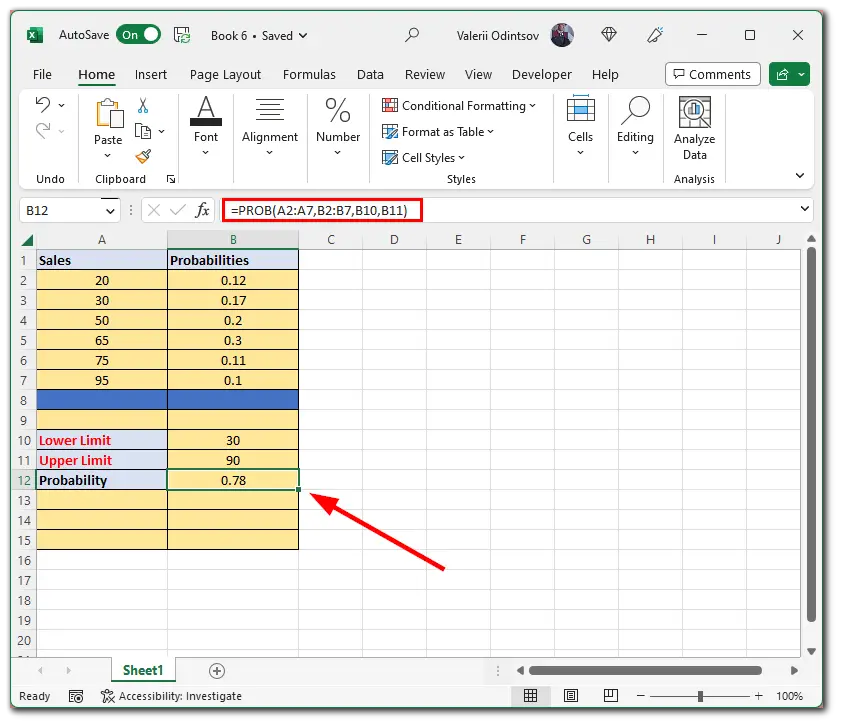

• A2:A7 is the range of events (sales) in numerical values.
• B2:B7 is the probability of getting the corresponding number of sales.
• B10 is the lower limit.
• B11 is the upper limit.
• In the end, you can see the result. The formula returned a probability value of 0.78 in cell B12.

You can also reduce the upper limit. Once you do this, the probability value will change. Moreover, you can show the probability as a percentage. Follow these steps:

• Go to the Home tab and click on the Number option.
• Then click on the Percentage icon.

As you can see, the probability is now shown as 37% considering that I have reduced the upper limit.

How to calculate dice probabilities in Excel

The coin flip example would be too simple to calculate in this situation. After all, you only have two sides there. Therefore the probability of one side being rolled is 50%. So let’s look at the dice example.

I’ve made a sheet that lists all the possible combinations that can come out of a two-dice roll. This is what it looks like:

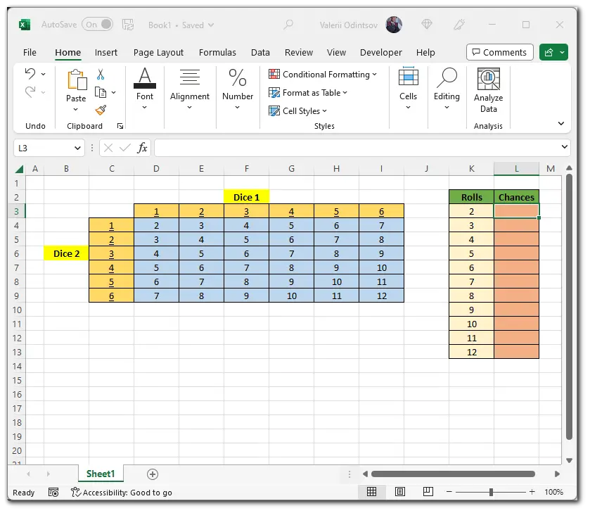
Now let’s calculate the probability of getting each amount in the table. Of course, you can calculate everything manually, but it’s much faster to do it with a formula. Why not use the Excel functionality when you can? Here’s what the formula looks like:

=COUNTIF([Cells_Range], [digit you want])

So I selected the L3 cell and entered:

=COUNTIF($D$4:$I$9, K3)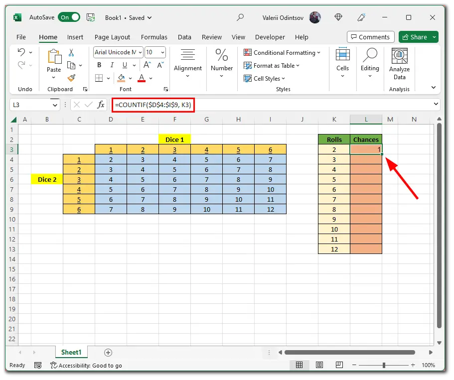

Then I apply this formula to all cells in the Chances column by dragging down this little square. And here’s the result:

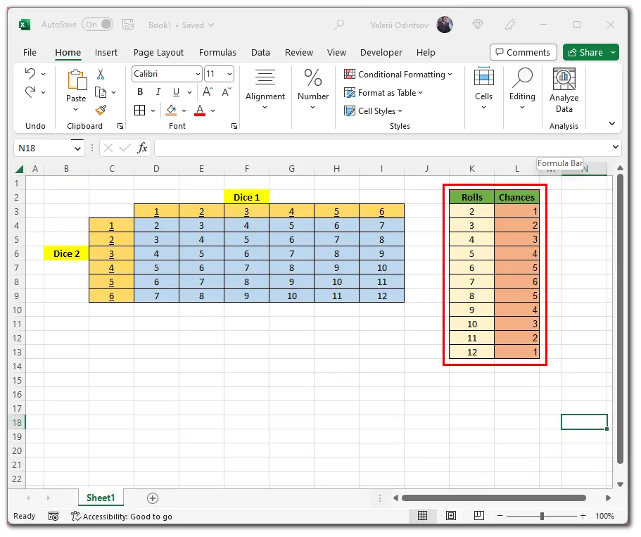
Next, we need to calculate each combination’s probability of rolling out. To do this, divide the number of chances of the combination rolling out by the maximum number of possible options, which is 36.

So let’s add one more column called Probability. Here select the M3 cell and enter:

=L3/36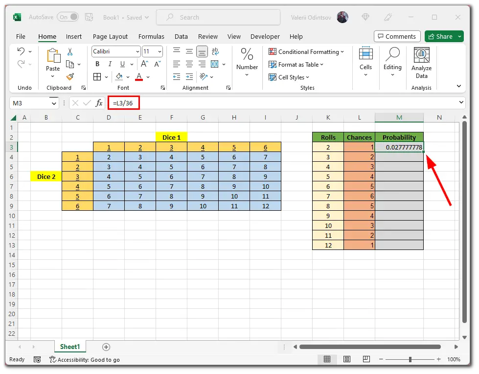

Now, apply it to the whole Probability column. And here’s what you should get:

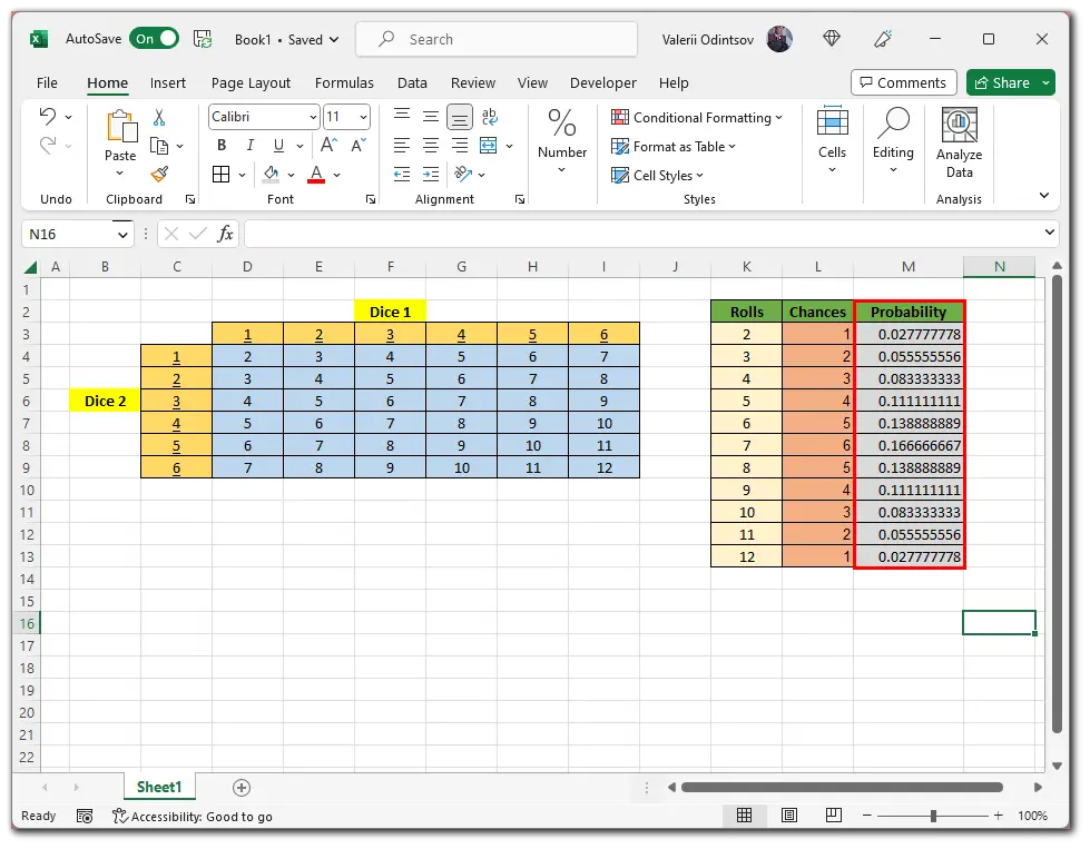
After that, you can turn on the percentage function, as shown above, for a clearer perception. Once we’ve done that, let’s use the PROB function to determine what combination has, for example, a better chance than 8.

So in our case, we have two limits:

• lower – 9
• upper – 12

You can assign them to specific cells, as in the first example, or type them in manually. There is really no difference.

Now, I select the M18 cell and enter the following PROB formula:

=PROB(K3:K13, M3:M13, 9, 12)

Finally, I just set the percentages to make it more convenient to read, and here’s the result.

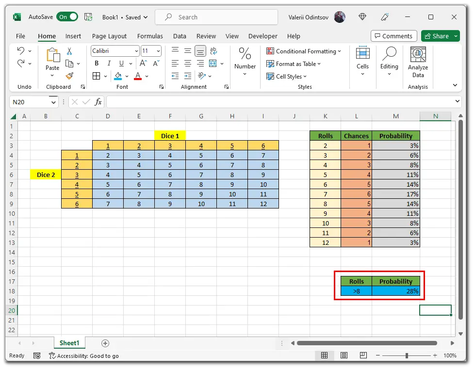
That’s it. We have successfully calculated the combination probability above 8, which is 28%. Frankly, this is one of the easiest methods to understand how to calculate the probability. Now, you can build on this example when calculating more complex cases. Good luck!