If you want to how to set up row fill color alternation and automatically highlight every other row or column on your worksheet, there’s a simple way to do this.

How can you add colors to alternating rows in Excel

Highlighting rows or columns in Excel with alternating fill colors is a common way to make the contents of a worksheet clearer. In a small table, you can select rows manually, but the task becomes much more difficult as the size of the table increases. It would be very handy if the color of a row or column changed automatically.

Well, here’s how you can add colors to alternating rows in Excel.

How to alternate row colors in Excel

When you need to color every other line in Excel, most specialists immediately think of conditional formatting and, after some time of fiddling with an intricate combination of MOD and ROW functions, achieve the desired result.

Alternatively, if you don’t want to spend tons of time and inspiration on a little thing like coloring in striped Excel spreadsheets, you can use a quicker solution – built-in spreadsheet styles.

The fastest and easiest way to customize the coloring of rows in Excel is to use ready-made table styles. In addition to other benefits (such as an automatic filter), color alternation is also applied to table rows. To convert a range of data into a spreadsheet, follow these steps:

• Select the range of cells in which you want to adjust the alternation of row colors.
• On the “Insert” tab, click “Table” or press “Ctrl + T”.

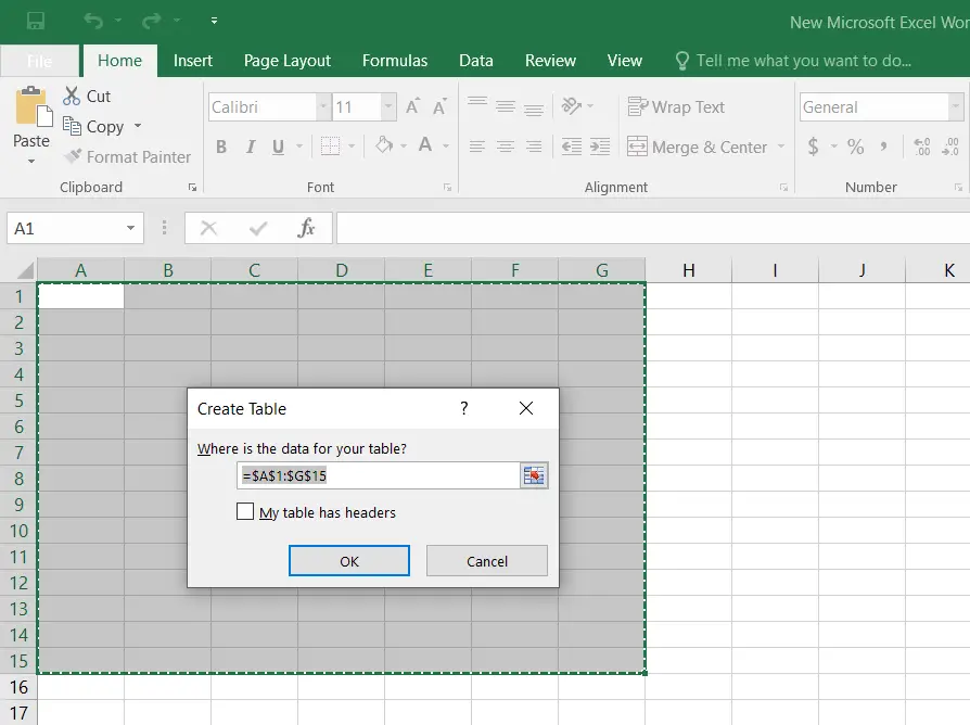
• Finally, click “OK”.

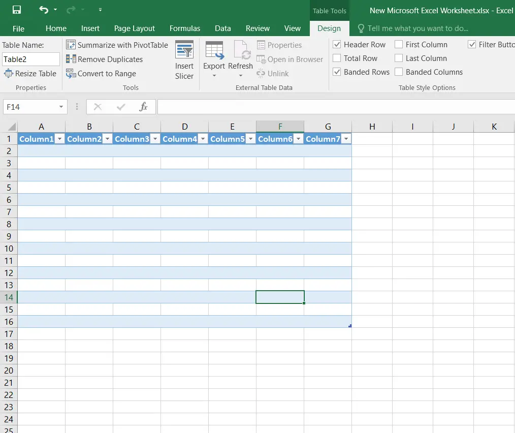
The even and odd rows of the created table are colored differently. And, remarkably, the automatic color rotation will be preserved when sorting, deleting or adding new rows to the table.

If you don’t need all the benefits of a table, and just want to keep the alternating coloring of the rows, the table can easily be converted back to a regular range. To do this, right-click any table cell and choose “Table”.

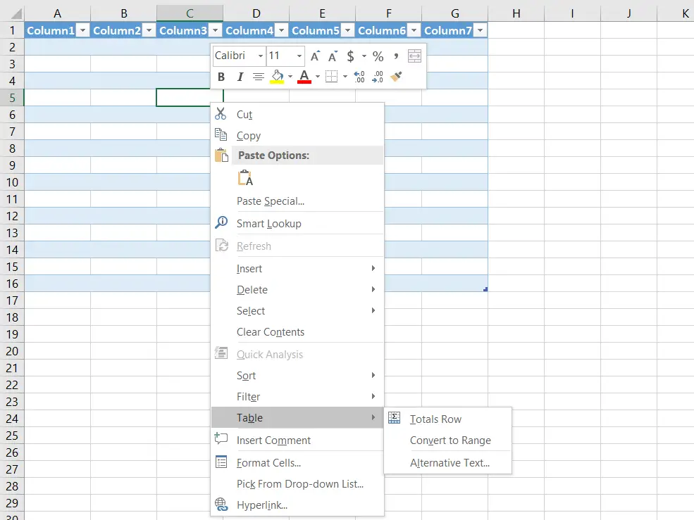
Then click on the “Convert to Range” option in the context menu.

If you decide to convert the table into a range, the color striping will not change automatically when new rows are added to the range. There’s another drawback: when you sort the data, i.e. when you move cells or rows within the selected range, the color bars will move along with the cells, and the neat striping will move completely.

How to choose your own colors for rows in Excel

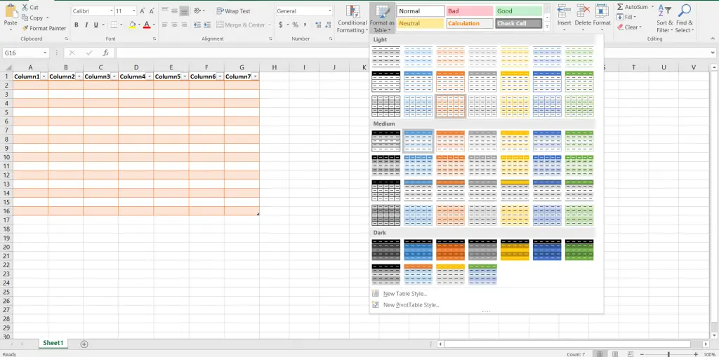
If the standard blue-and-white Excel spreadsheet palette doesn’t appeal to you, there are many templates and colors to choose from. Simply select a table, or any cell in that table, and then on the “Home” tab under “Styles”, select the appropriate color. Alternatively, you can click “Format as Table” and select the design you like.

How to select different number of rows in table bars in Excel

If you want to select a different number of rows in each of the colored bands in the Excel sheet, for example, to color two rows with one color and the next three with another color, you need to create a custom table style. To do so, you have to follow these steps:

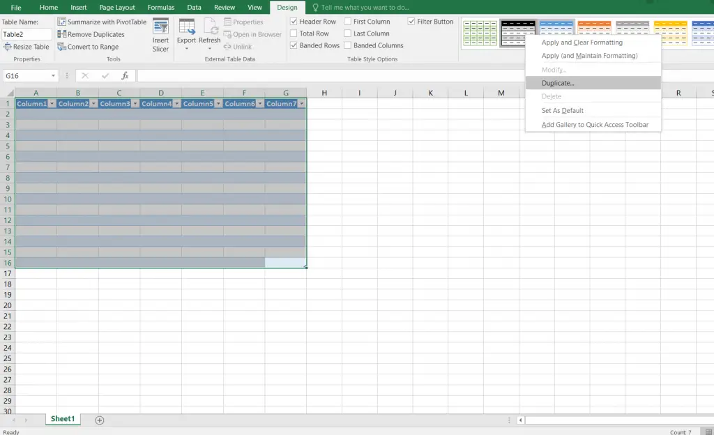
• Open the “Design” tab, right-click on the table style you like and click “Duplicate” in the menu that appears.

• In the “Name” field, enter the appropriate name for the new table style.
• Select the “First Row Stripe” item and set the “Stripe Size” to 2 or any other value you prefer.

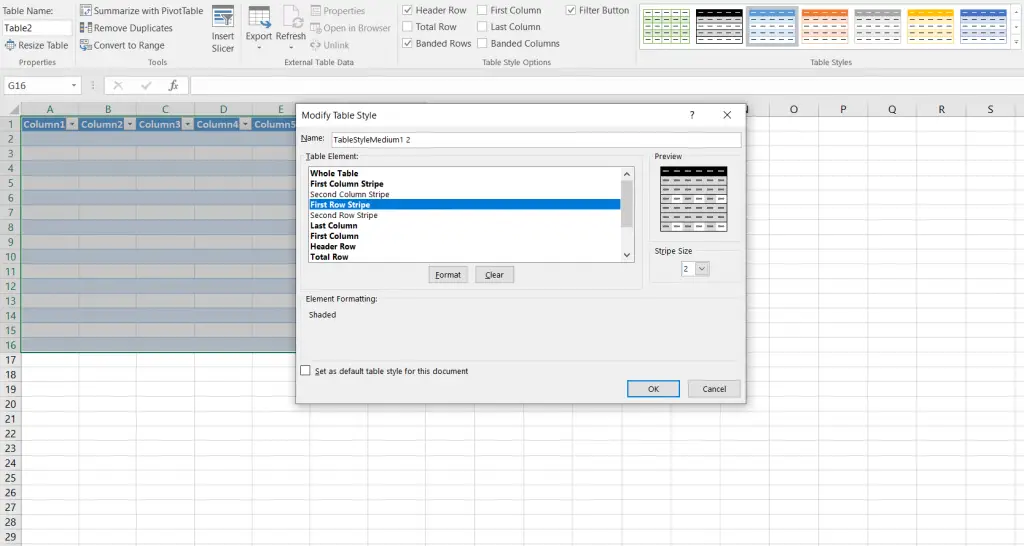
• Next, select the “Second Row Stripe” element and repeat the process.
• Click “OK” to save the custom style.
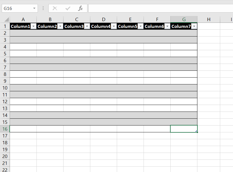
• Select the style you just created in the “Table Styles” gallery. The created styles are located at the top of the gallery in the “Custom” section.

If the created style isn’t quite as desired, it can always be easily changed.