Microsoft Excel is designed in such a way that it’s convenient not only to enter data into the table, edit them according to a given condition but also to view large blocks of information. This is why Excel allows you to freeze rows and columns.

How to anchor rows and columns in Excel

Thanks to Excel’s high performance, you can store and work with data in millions of rows and columns. However, scrolling down through all those many cells, by 10,000 rows, it’s easy enough to lose the connection between the values in those cells and their meaning. This is one of the reasons why Excel has prepared a special tool for you called Freeze.

This tool allows you to scroll through cells with information and see the row and/or column headings that are fixed and cannot scroll with the rest of the cells.

Well, here’s how to freeze rows and columns in Excel in a few easy steps.

How to keep headers visible in Excel

If you have an ordinary table with one row in the header, the steps are very simple:

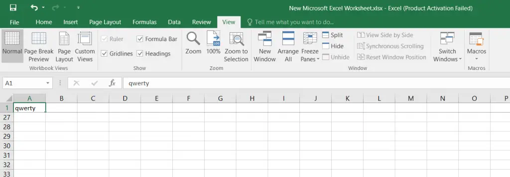
• Look at the top row of headers and make sure that this row is visible. You don’t need to highlight the line itself.
• Open the “View” tab in Excel and look for the “Freeze Panes” command icon in the “Window” group.
• Click the small arrow next to the icon to see all the options.

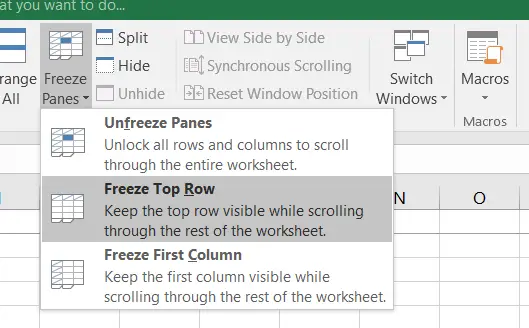
• Select the “Freeze Top Row” option or “Freeze First Column”, depending on how you want to organize your data.

Whenever you anchor rows or columns, the Freeze Panes command turns into the “Unfreeze Panes” command, which allows you to quickly unlock rows or columns.

How to pin multiple rows and/or columns in Excel

More and more often, you may come across tables that have multiple rows in the header. These are complex structures, but they allow you to put more detailed text in the headers, thereby describing the data in the table more clearly.

In addition, the need to anchor multiple rows arises when you want to compare a certain area of data with another area that is several thousand rows below.

In such situations, the “Freeze Top Row” command isn’t going to be very useful. However, being able to lock an entire area at once is what you really need.

Here’s how you can do it:

• This is the key point. Select the cell below the rows and/or to the right of the columns you want to anchor.
• Open the “View” tab and look for the “Freeze Panes” icon in the “Window” command group.
• Click the small arrow next to the icon to see all the options and select “Freeze Panes”.

Many novice users often complain that this technique doesn’t work for them. This can happen if you have previously fixed an area.

If any of the rows or columns are already anchored, you will see Unfreeze panes instead of Freeze panes. Look at the name of the command before you try to unfreeze panes and it will work just fine.

Use this small but very handy tool to keep the area headers visible at all times. That way, when you scroll through the sheet, you’ll always know what data is in front of you.

How to anchor a row and a column at the same time in Excel

If you want to freeze a row and a column at the same time in Excel, you have to follow these steps:

• Make active the cell at the intersection of fixed rows and columns. It should be immediately below the desired rows and to the right of the desired columns.
• Then, open the “View” tab and look for the “Freeze Panes” icon in the “Window” command group.
• Click the small arrow next to the icon to see all the options and select “Freeze Panes”.

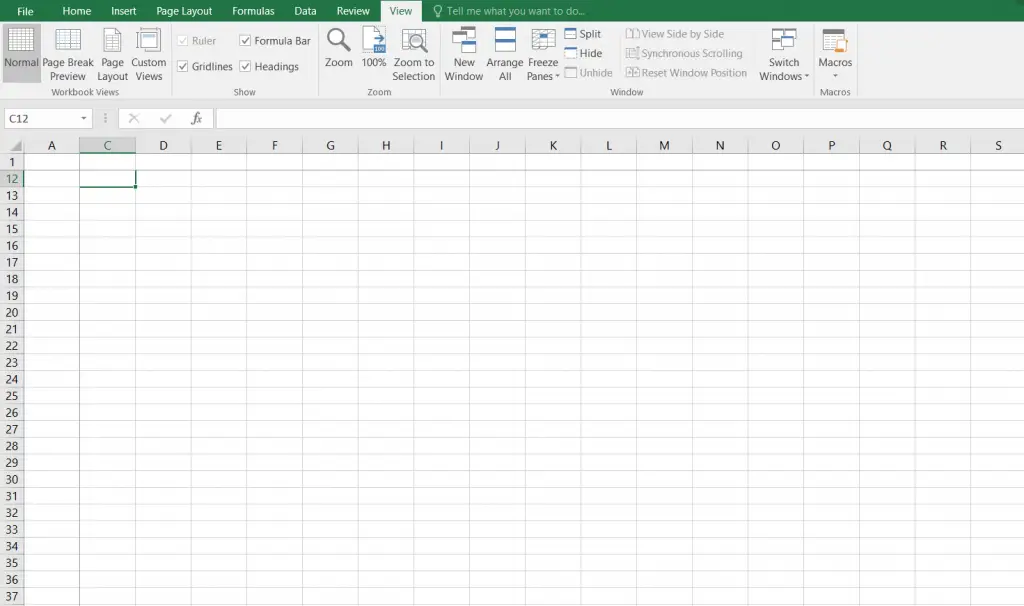
In the image, you can see that when you scroll, the highlighted areas remain in place.