Today, working with tables doesn’t take the last place in various spheres of office work and not only. Many companies specifically buy whole complexes of text editors, which have the ability to create and manage tables, as it’s very convenient for storing and analyzing various data. Of course, everyone immediately thinks of Excel from Microsoft Office. However, there’s a more convenient and user-friendly spreadsheet editor. This is Google Sheets.

Google has created a more concise, technologically advanced, and usable version of spreadsheets, which is now used in various professional fields, including marketing and SMM. And it’s all for a reason because Google Sheets has all the same functions as Excel. However, they are much easier to use. One of these functions is the counting of non-empty cells. Well, let’s take a closer look at how you can count non-empty cells in Google Sheets.

What are the main benefits of Google Sheets?

Google Sheets is a free IT product from Google that works without tethering to a desktop PC. This means that all your documents are saved in the cloud, and you can access them at any time when you have an Internet connection. In addition, your documents are automatically saved after any change, so you can relax and not have to press “Ctrl + S” every 5 minutes like in Excel to avoid losing precious data.

Here are the main benefits:

• Real-time analytics wherever you are.
• Editing, formatting, and commenting by any user who has access to the spreadsheet via a link.
• You can see the changes you made before. It’s possible to roll back to any point where you need to make new data, change the formula for calculations, add a column, etc.
• There’s no need to send files by e-mail to customers or contractors or do extra work to download the document, open it, or save changes in it.
• The document won’t disappear, you cannot delete it accidentally. If you delete it, it’s stored in the “Trash” folder for 30 days and can be restored at any time.
• You can import data from other available sources without losing functionality.

After all, if you’ve worked with Excel before, it shouldn’t be hard to get used to Google Sheets quickly.

Read Also:

• How to name columns in Google Sheets
• What is today’s date formula in Excel and Google Sheets
• How to insert a checkmark in Google Sheets

How to use the COUNTA method to count non-empty cells in Google Sheets

When using Google Sheets, there may be situations in which cells aren’t filled with any data. In such cases, you might want to count the number of such cells. This is possible with the Google Sheets “COUNT” functions.

The first function you should know about is COUNTA. The COUNTA is used to count non-empty cells, but it has one drawback. Sometimes the COUNTA function doesn’t capture hidden special characters. So, in Google Sheets, the COUNTA function counts the number of cells in a range that contain values or a text string. It ignores empty cells when counting.

Well, if you want to count the number of the not blank cells, you have to follow these steps:

• First of all, select a blank cell and type the “=COUNTA” function including the range of cells that you want to count. As an example, I use “=COUNTA(A2:A5)”.

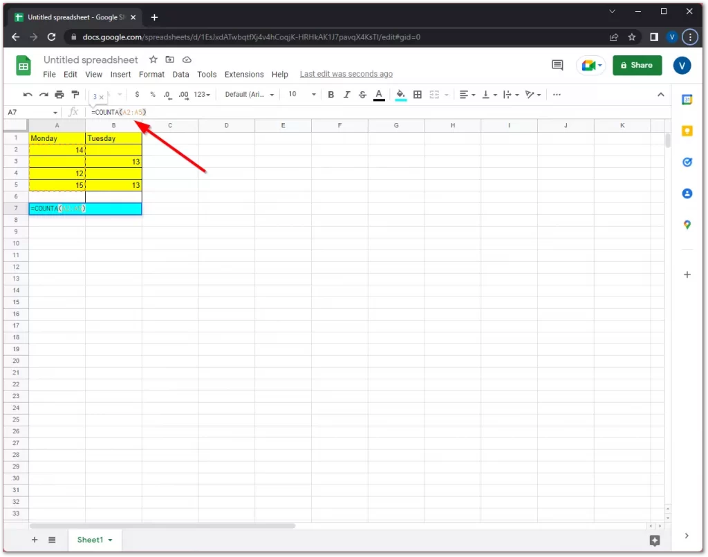
• After that, press Enter, and the “COUNTA” function will automatically count non-empty cells.

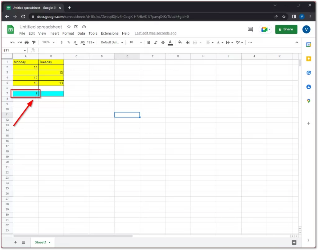
• Finally, you should have the number of cells that have values in them.

Once you have completed these steps, you will be able to count non-empty cells in Google Sheets using the COUNTA method. In fact, everything isn’t as difficult as it seems, and even easier than, for example, creating a Gantt chart in Google Sheets.

How to use the SUMPRODUCT method to count non-empty cells in Google Sheets

Unlike the COUNTA function, the SUMPRODUCT function has the property of detecting hidden special characters. So it will do an even better job of counting the number of cells you need. Here’s how you can do it:

• Select an empty cell and enter the function “=SUMPRODUCT(–(LEN(range)>0))” to count cells that don’t appear empty. I use “=SUMPRODUCT(–(LEN(B2:B5)>0))”.

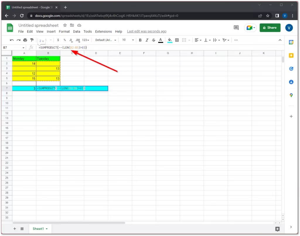
• When you do this, the LEN function returns a value that’s greater than zero, counting the number of characters that appear on the sheet.
• Then, just press Enter, and the number of the non-empty cells will automatically appear.

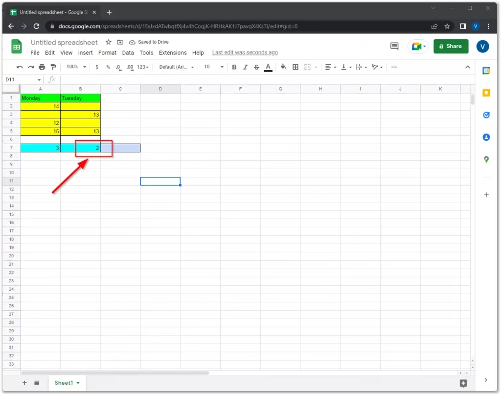
Once you have completed these steps, you will be able to count non-empty cells in Google Sheets using the SUMPRODUCT method. Moreover, you can also hide these cells from the specific people who also have an access to your spreadsheet in Google Sheets.

How to use the COUNTIF method to count non-empty cells in Google Sheets

Google Sheets hides some special characters from view because of their special functions. These include, for example, the apostrophe, which is used to indicate that numeric characters should be interpreted as a string.

To solve this problem, you can use the COUNTIF function to count cells that aren’t empty and in which special characters aren’t hidden. To do so, follow these steps:

• Select an empty cell and enter the function “=COUNTIF([range],”>0″&”*”)” to count cells that don’t appear empty. I use “=COUNTIF(A2:B5,”>0″&”*”)”.

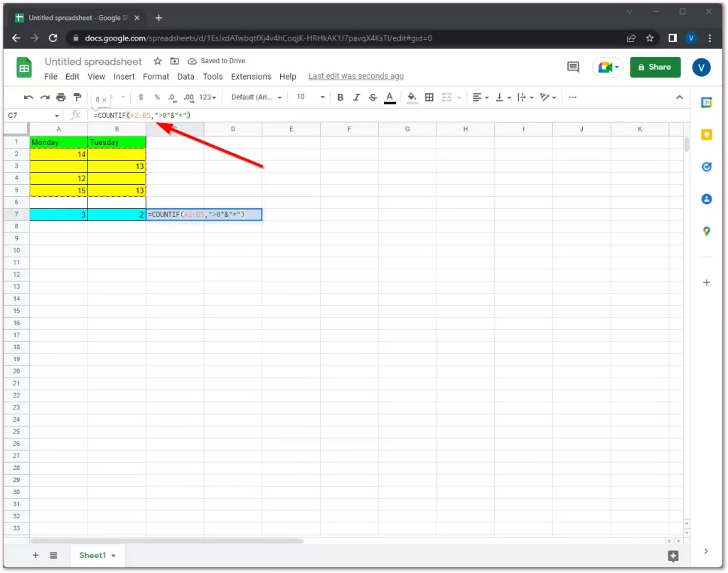
• “>0″&”*” is a condition for sifting out cells that contain hidden characters, so only those with letters and numbers are counted.
• Finally, just hit Enter and the number of the non-empty cells will automatically appear.

Once you have completed these steps, you will be able to count non-empty cells in Google Sheets using the COUNTIF method. Such actions can be also performed using, for example, a master sheet in Google Sheets. This doesn’t change the conditions of the functions in any way.

Read Also:

• How to use the slicer in Google Sheets
• How to print a Spreadsheet in Google Sheets
• How to add handwritten signature to Google Docs

What does conditional data formatting mean in Google Sheets?

The easiest way to change the display of a cell is through the options in the Control panel at the top. Here you can change the appearance of fonts, borders, paragraphs, and text transfer rules. Manual tools aren’t always sufficient. Conditional formatting is used for automatic adjustments. For example, you can set all cells to be the same size in your Google Sheets document.

The rules are set for:

• Individual rows and columns.
• Cells or ranges.
• The whole table.

You can set them up through the Format section. Conditions are added in this window, for example, at certain values cells are repainted in a given color. You can change not only the appearance but also the text style.

You can use complex rules for highlighting. For example, you run more than 100 advertising campaigns. It’s impossible to check each of them manually. Suppose you need to mark the most effective of them, in terms of targeted actions. To do this, you can create complex rules with the “Your Formula” option. In this case, when a certain conversion value is reached, the content is marked.

When you need to visually analyze a range where numbers need to be graded, it’s most convenient to use a gradient fill.