
Google Sheets is an extremely convenient online resource for creating all kinds of documents in spreadsheet format, storing them, and distributing them. With all the features of Microsoft Excel, while not requiring a PC download, this service has quickly replaced the downloadable Excel program for many people. However, even experienced Microsoft Office users sometimes need help to figure out how some features of Google Sheets work.
How to freeze rows
Sometimes when making tables, people need to change the name of a column. Columns have capital letters from A to Z as names. These names cannot be changed in any way.
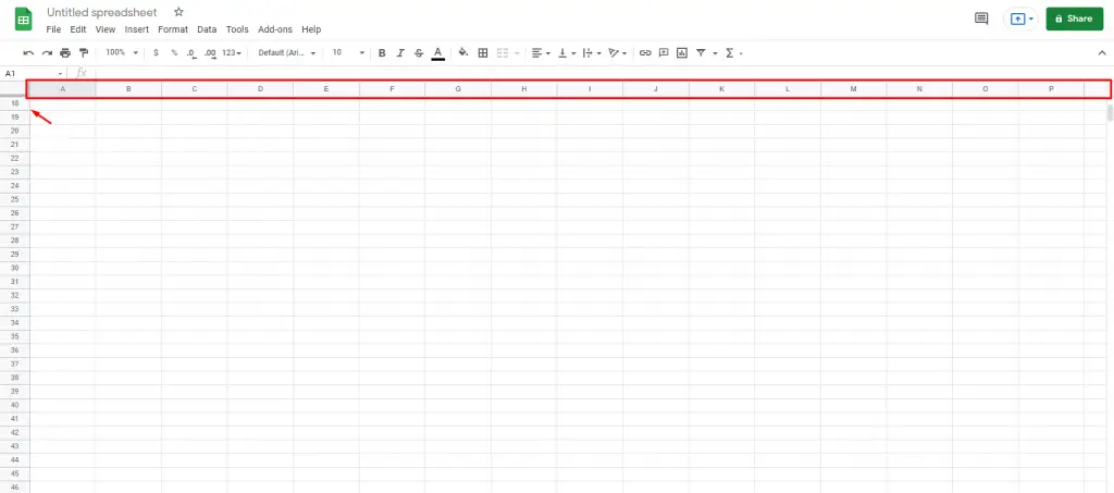
Whatever you do, these names will always stay the same and stay at the top of the table, no matter how far down you scroll. However, instead of changing these designations, you can add your headings to the first row and freeze them. It’s pretty easy to do, it requires:
1. First, open the file with the table you want to make adjustments to.
2. Once it loads first, click on the number in front of the first row.
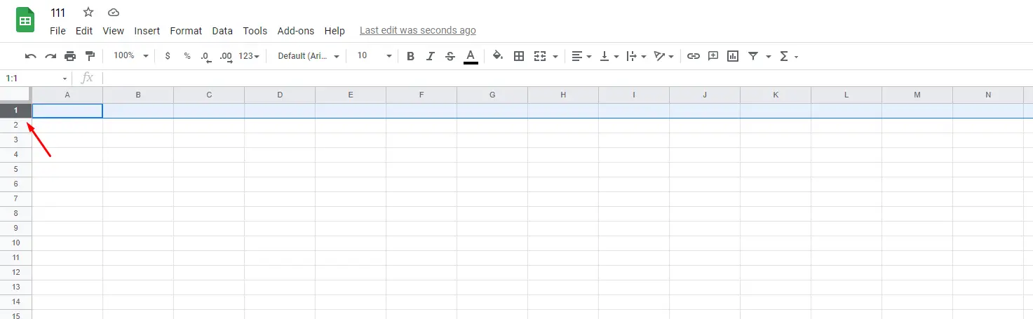
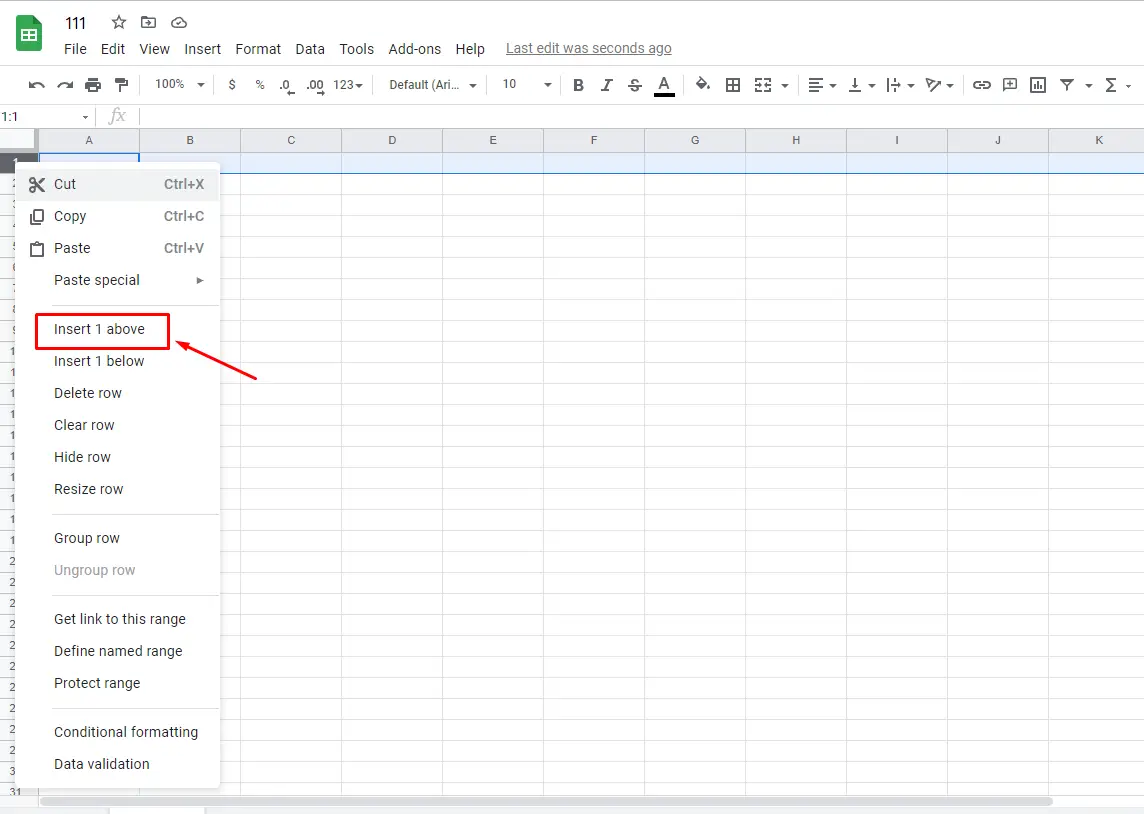
3. If the row you need isn’t empty, right-click on the number in front of the row and choose Insert 1 above.
4. Highlight the cells where you want to put the title and type the desired title in them.
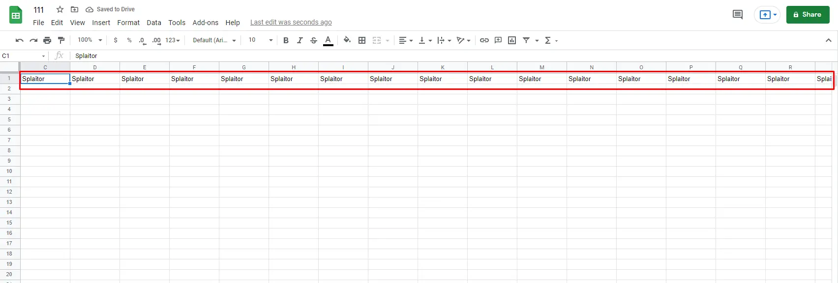
5. Next, click the number in front of the first row again.
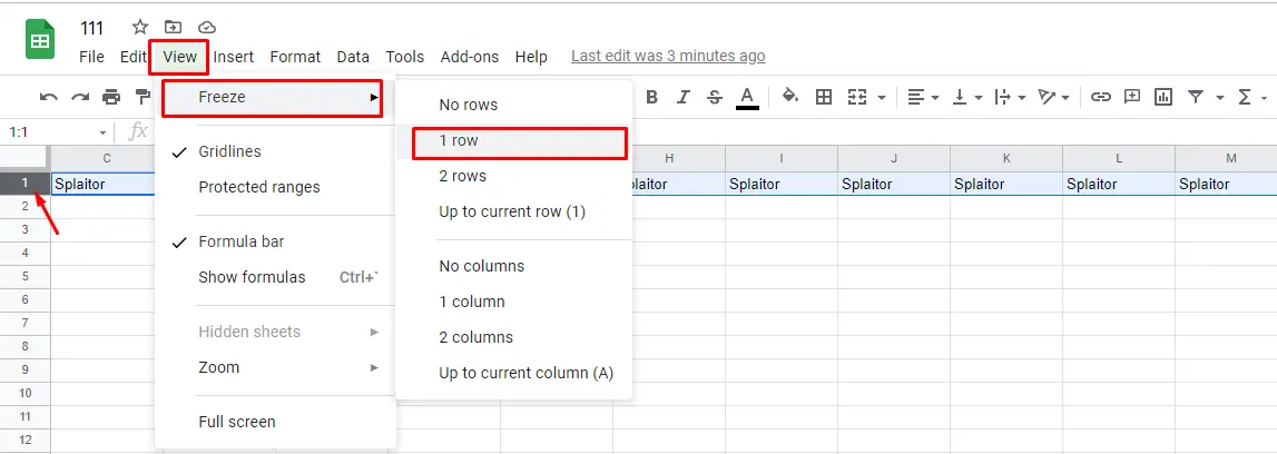
6. In the functions at the top of the screen, click on “View”.
7. When the window opens, select “Freeze”.
8. After this, another menu will appear. Select “1 row”.
If you did everything correctly, the row with the column names is now frozen. You can scroll down as much as you like, but you will still be able to see the column names at the top. If you enter a separate set of names in the second or third row, and you want them to always stay at the top of the table, repeat these steps above towards those rows.


