Today there are a huge number of different tools for working with texts, various data, and information in general. All ordinary Windows users have definitely heard of or used such a tool for working with data as Microsoft Excel. If you’re one of these people, then you should know that programs of this type are really needed in the work of, for example, an online marketer or any other specialist. However, quite often there’s a question of using the capabilities of a particular service on different devices. Google Sheets is the leader in this regard.

However, not all Google Sheets users know how certain features of the service work. For the most part, all of its functions are easy to implement. So, if you need to create a master sheet in your Google Sheets document, here’s how you can do it.

What is a Google Sheets service?

Google Sheets is essentially Google’s equivalent of Microsoft Excel. It’s suitable for almost the same functions, namely: working with a lot of information, lists, checklists, and reports. This tool has a huge number of different features, ready formulas, and logical functions to work with text, graphic and tabular data in one month.

It’s even easier when you realize that to use this service, all you need is a personal Google account and a web browser. After all, Google Sheets is a web application and all you need to access it’s an Internet connection. You may have experienced situations when large amounts of information in Microsoft Excel make your PC or laptop (if they’re weak) slow and glitchy. With Google Sheets, there should be no such problems. Also, don’t forget about the automatic saving of the document in the aftermath of any change.

Well, if you run into the problem of creating a master sheet in Google Sheets, you have to know that, frankly, there’s nothing complicated about it, just as there’s nothing complicated about using some functions in Excel. So, don’t stop and keep reading.

Read Also:

• How to insert check mark in Google Sheets
• How to set the print area in Google Sheets
• How to make a Gantt chart in Google Sheets

What is a master sheet in Google Sheets?

Well, as you may have read above, Google Sheets has many useful features, for example, a dark mode. One of them is also the ability to create a master sheet and then attach secondary sheets to it.

What exactly can you do with a master sheet in Google Sheets? The first and most basic thing is to synchronize multiple sheets into one master sheet, which will automatically update. One reason you might find this helpful is to import historical stock data. You can even make spreadsheet analysis more efficient by adding color-coded drop-down lists and finding duplicate values in multiple columns.

This is a great option if you have several people working with different spreadsheets and you want to compile the data into one spreadsheet for review. Instead of having to redo the work you’ve already done, you can easily pull data from other spreadsheets and automatically update the cells. The main thing is then also don’t forget to configure Google Sheets so that your document doesn’t open on the wrong sheet.

It’s very simple – when someone makes changes to one spreadsheet, those changes can automatically be reflected in the master sheet. That’s what makes this Google Sheets feature so cool.

How to make a master sheet in Google Sheets

You have to be aware that you can combine as many sheets as you want and need. I will show you an example of how to combine two secondary sheets with one master sheet.

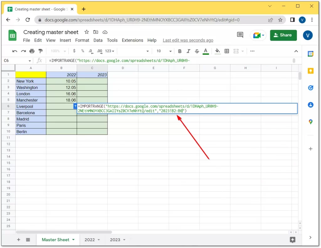
First of all, you need to open all the sheets you want to combine in their own tabs. You will need to take information from each table for the merge to work on the master table, so all tables must be open. The formula you have to use to get these results is the “=IMPORTRANGE” formula. This is what is required of the function:

• =IMPORTRANGE(spreadsheet_url, range_string)
  • spreadsheet_url is a link to the spreadsheet from which you want to take the data. It should always be enclosed in double quotes.
  • range_string refers specifically to the cells that you want to enter in the current sheet.

It has several different elements that need to be set up for your spreadsheet. So, follow these steps to continue:

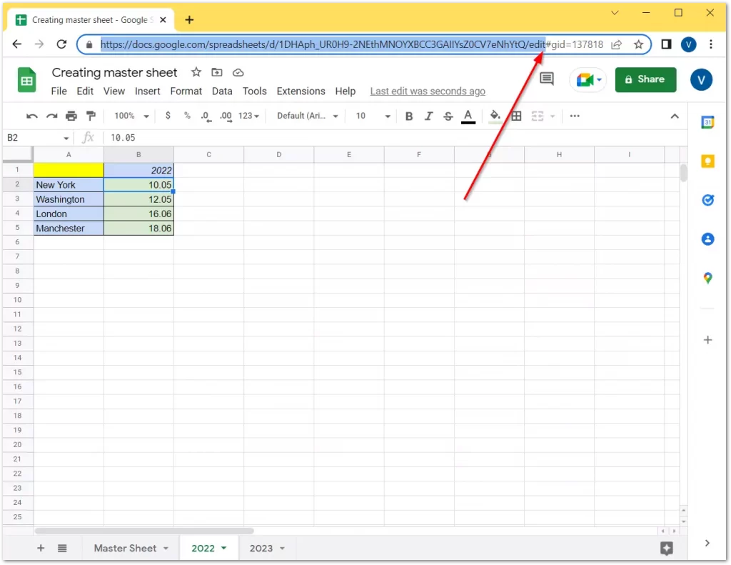
• Open the sheet from which you want to extract data.
• Then, click on the URL bar and copy the link to this file right till the hash “#” sign.

• Go back to the spreadsheet you want to add information to, type “=IMPORTRANGE” where the borrowed table should appear, and insert the link as the first argument.

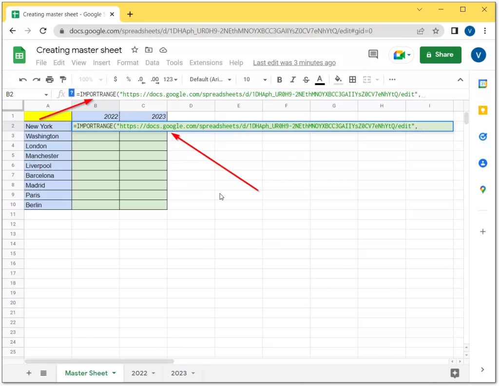
• After that, separate it from the next part with a comma.
• In the second part of the formula, enter the name of the sheet and the exact range you want to draw.

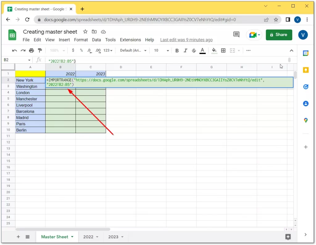
• Confirm by pressing “Enter”.
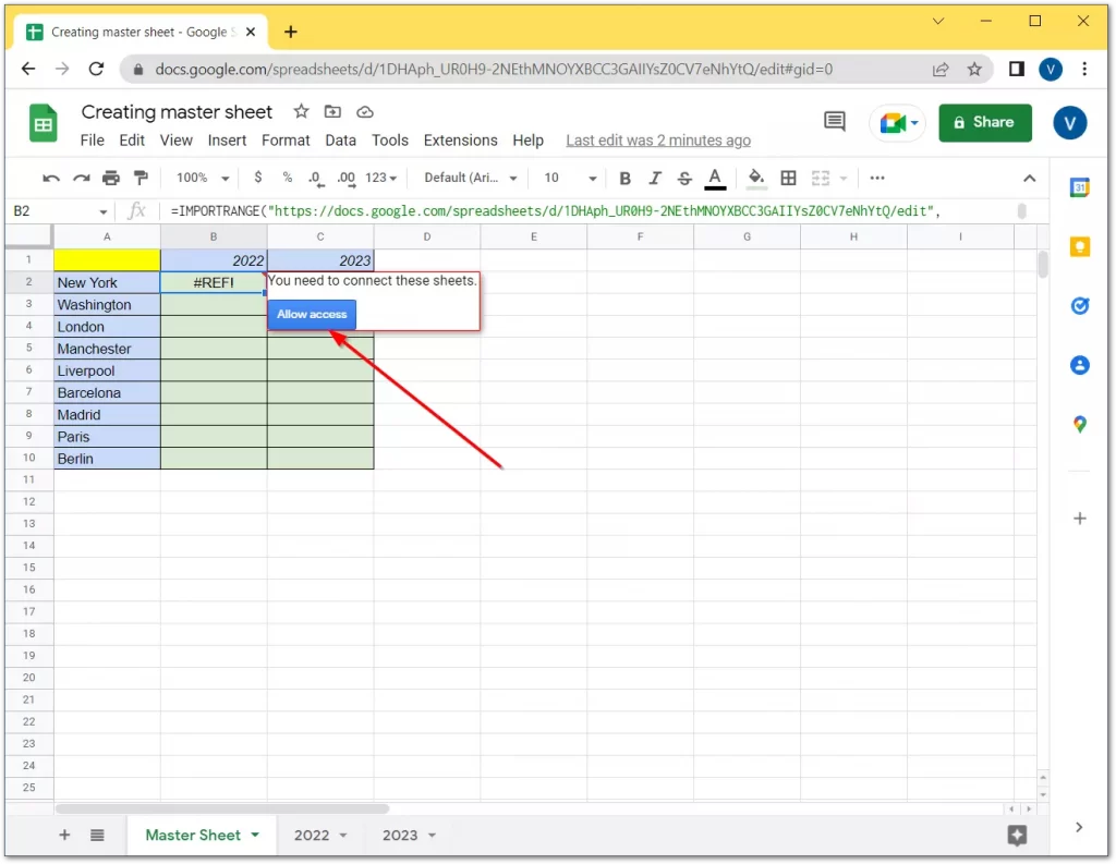
• Although the formula looks ready now, it will return a “#REF” error from the beginning. This is because the first time you try to extract data from any spreadsheet, “IMPORTRANGE” will request access to it. Once permission is granted, you can easily import records from other sheets in that file.
• So, click on the “Allow access” button.

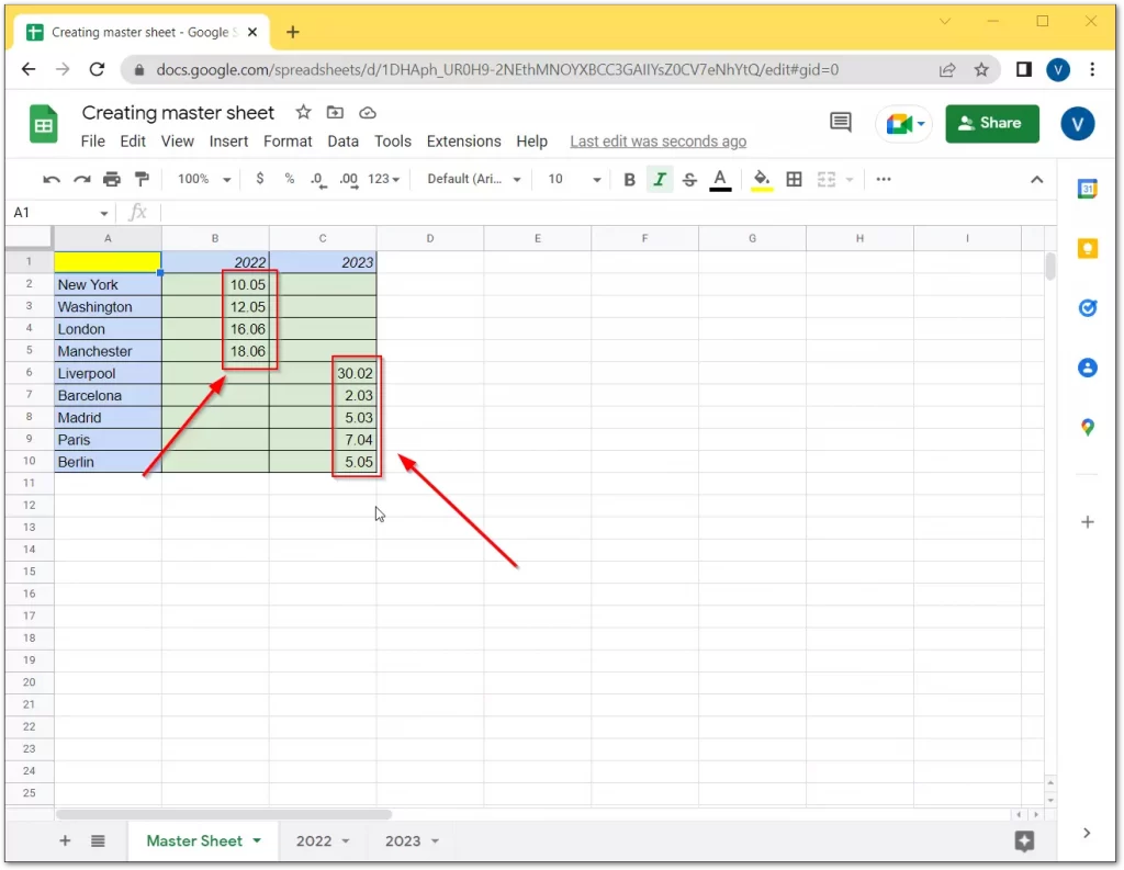
• Now, you can see that the master sheet is filled with data from the first secondary sheet (“2022”).
• Next, just do the same steps to the second sheet (“2023”).

• Finally, you should get a full result as in the screenshot below.

Remember that you have to be very careful when setting up a range. After all, one little mistake can ruin the whole process.

Once you have completed your spreadsheet, you can also copy it to another workbook in Google Sheets.

How does a Combine Sheets add-on work?

If the standard ways of combining data from multiple sheets in Google Sheets seem boring to you and the features put you off, there’s a simpler approach. You can try to use a special add-on called Combine Sheets which was designed to import data from multiple sheets to a master one.

So, if you want to use a Combine Sheets add-on to merge data, you have to follow these steps:

• First of all, you have to install the add-on. You can do it by following this link.
• Just click on the “Install” button and follow the instructions.
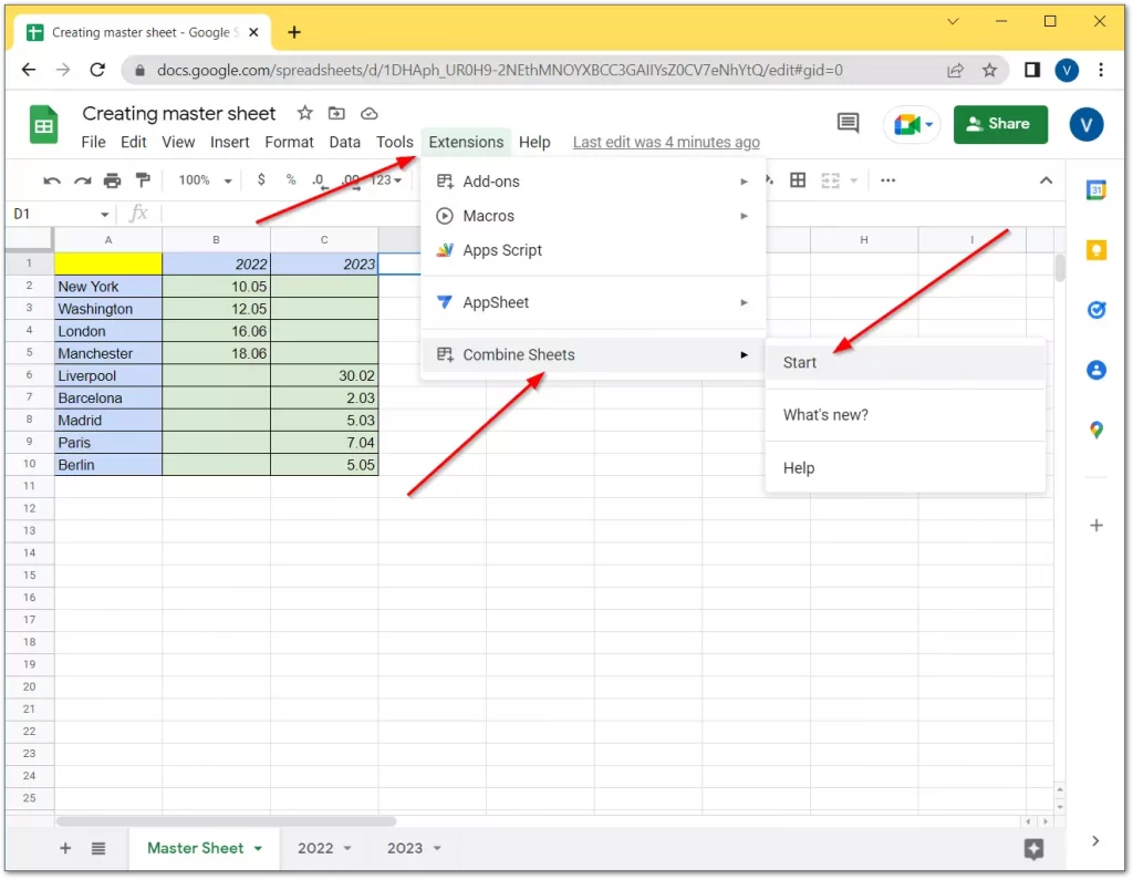
• After that, click on the “Extensions” tab, select “Combine Sheets” and click “Start”.

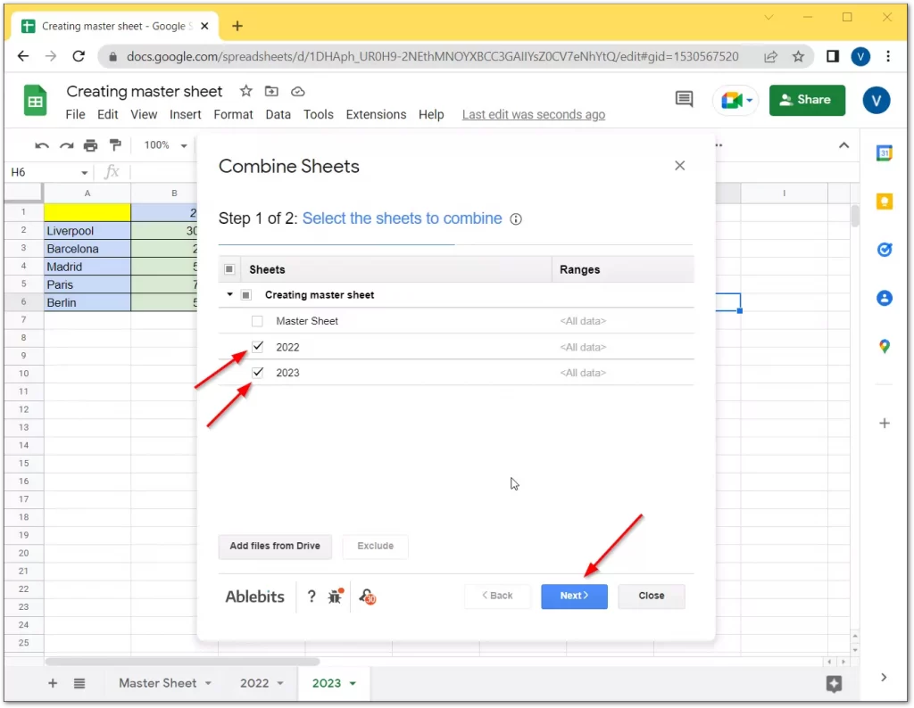
• Choose all needed sheets and click on the “Next” button.

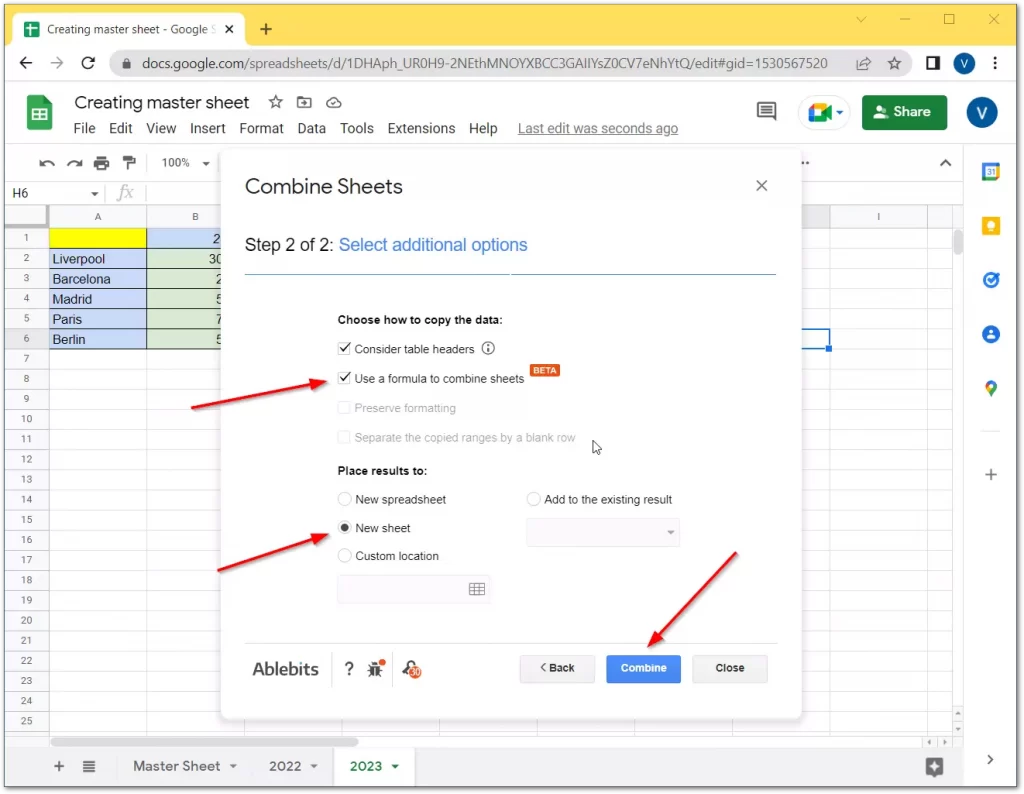
• Select how you want to receive the data:
  • as a formula. Check the “Use a formula to combine sheets” checkbox if you want the master sheet to change dynamically depending on the original content.
  • as values. If manual editing of the resulting table is more important, ignore the above parameter and all data will be merged as values.
• Now, check the “New sheet” checkbox and click “Combine”.

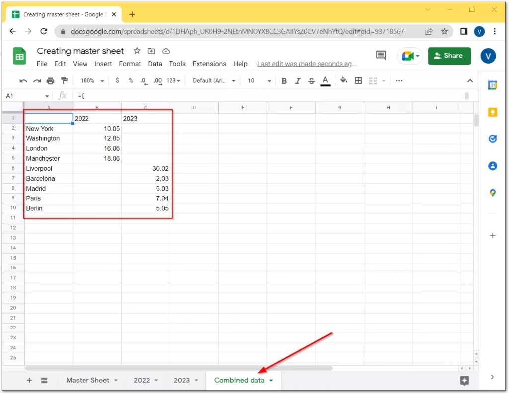
• Here’s a new sheet with combined data from the secondary sheets you have selected.

Of course, your spreadsheets can be much larger, and you can combine many different sheets as long as the resulting spreadsheet does not exceed the 5 M cell limit. Moreover, you can also hide the cells that you don’t need anymore.

Read Also:

• How to fix Google Sheets formula parse error
• How to use the slicer in Google Sheets
• How to make Google Sheets columns to be the same size

What are the main hotkeys in Google Sheets?

If you learn and automate the use of at least a third of hotkeys, you can increase the speed of work in Google Sheets by 1.5 times. The service supports more than a hundred hotkeys. Here are a few of the most useful for Windows:

• “Ctrl + Spacebar” – select a column.
• “Shift + Spacebar” – select a row.
• “Ctrl + Enter / D / R” – fill range / down / right.
• “Ctrl + K” – insert reference.
• “Home” – go to the beginning of the line.
• “Ctrl + Home” – go to the beginning of the sheet.
• “Ctrl + Backspace” – move to the active cell.

Google Sheets also has common Windows and Mac shortcuts for standard actions – copy, paste, cut, print, find, etc. For a complete list of keyboard shortcuts, see the Google Sheets Support web page.

You should also know that once you have finished editing your spreadsheets, you can always easily and simply print them out.