Google Sheets is one of the most popular spreadsheets and reporting platforms. It has quite a few different tools and competes quite well with its closest competitors. One of the handy features is displaying formulas instead of numbers in cells.
It will be especially useful for new users or to analyze a table you created a long time ago. This way you can see which formulas you used in specific cells. You can turn it on and off at any time using the View tab. It is also possible to do this for one single cell instead of the whole document.
How to show formulas in all Google Sheets cells
It would be most convenient to switch all cells at once to show formulas instead of specific numbers. As I wrote above, this will help you better understand exactly how the table works. For example, if you have an error somewhere, you will be able to understand which cells are related to the one that shows the error. To do this you need to:
- In your table, click on View in the toolbar.
- In the pop-up menu, hover your cursor over Show.
- Select Formulas to toggle the formulas display.
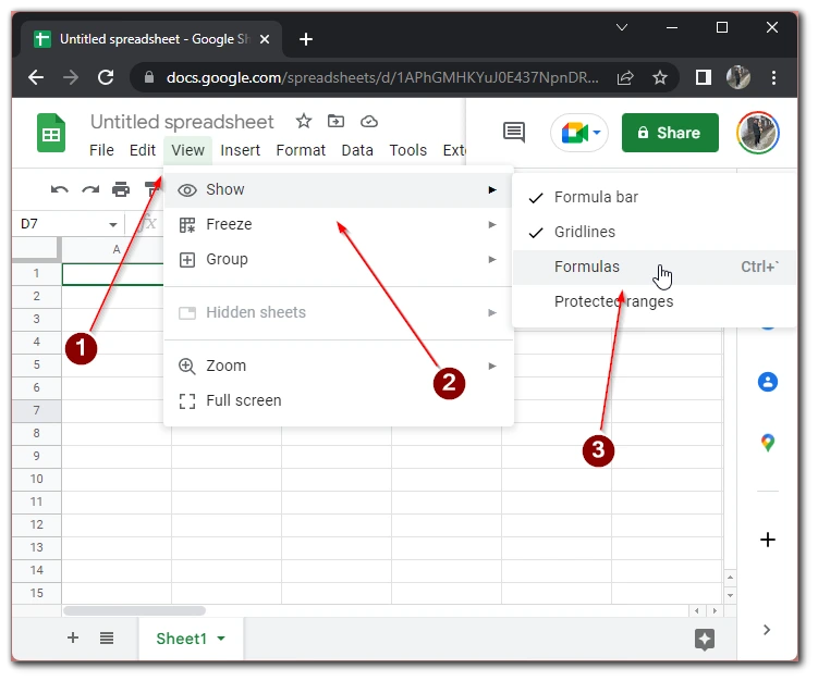
This will immediately switch the your table view. To switch back, you just need to repeat these steps. Note that this function will only show formulas, if you need to see links or other information, you’ll have to use other tools.
How to show formulas in a specific Google Sheets cell
In addition, you can demonstrate the formula in a particular cell. This will help you review the formula in a particular cell if you think it’s the problem. To do this you will need to:
- Select the cell with the formula.
- In the formula edit box, put a ‘ sign in front of the formula.
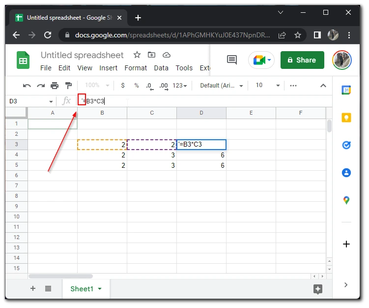
All formulas with this sign in front of them will be shown over the numbers in the cells. You can apply this method to any formula in Google Sheets. The main thing that you need to understand is that this sign must be before the equal sign, that is, before the beginning of the formula itself.
How to use a formula for an entire column in Google Sheets
You can also apply a formula to an entire column with just a few clicks. This is useful when creating a large table with reports, for example, or for products in an online store. To do this you need:
- Enter your formula in the top cell of the column.
- Click on the column name to highlight the entire column
- Press CTRL+D.
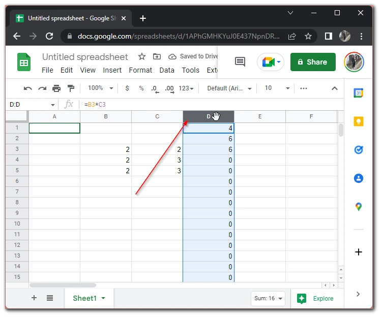
This will apply the formula to all cells in the column in your spreadsheet at once. You can also select a cell with a formula and click on the square at the bottom right and drag it down or up. This will apply the formula to all cells that you drag the mouse to.
Read also:
- How to start or join a Google Meet from Slides, Sheets or Docs
- How to count non-empty cells in Google Sheets
- What is the VLOOKUP function in Google Sheets and how to use it?
How to change the color of numbers less than 0 in Google Sheets
You can also use a special rule to specify all cells where the value can be less than zero. This will be especially useful in reports, when you can track the minus in the your finances calculation. You can do this by using formatting to do this:
- In your spreadsheet, click on Formatting, then select Conditional Formatting.
- From the pop-up menu, select the area where you want to apply this rule.
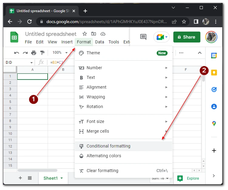
- Then select Less than from the Format Rule list. In the Value of formula field, enter 0.
- In the toolbar, select the fill color for the cells where there will be a negative value.
- Click Done.
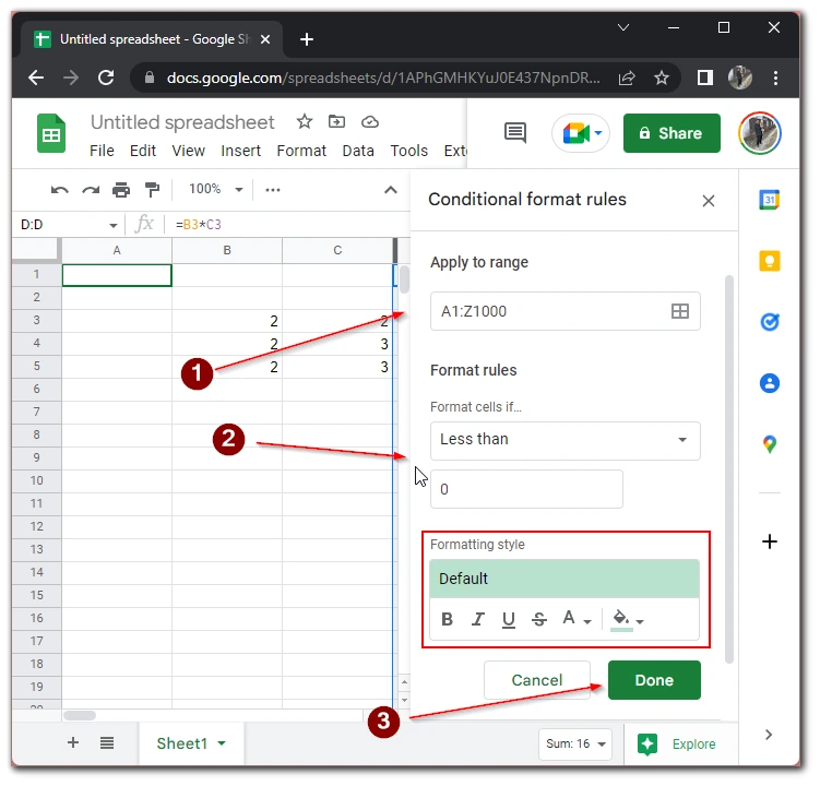
After this, the rule will be applied and all cells that match your rule will be filled with the desired color. In fact, there are quite a few different conditions that you can apply to your table to highlight the desired elements without having to parse the table manually.


