
Tables are quite handy for handling large data sets. Of course, the most popular type of spreadsheet is Excel. However, in recent years, users are increasingly turning to a spreadsheet service from Google, called Google Sheets. It’s a very convenient online service in which all your files automatically remain in the cloud. This service has quite a few different features that help you quickly process and explore large amounts of data.
For example, in order to find certain values in huge tables, users use the VLOOKUP function. This function is also available in Excel. At first glance, this function may seem quite complicated, but in fact, there is nothing complicated if you understand more.
What is the VLOOKUP function in Google Sheets
Google Sheets is a pretty handy service that has very rich functionality. In general, most of the features that were in Excel were also added to Google Sheets. The most convenient thing is that this service is also connected with all the other services of Google, such as Google Docs or Google Photos.
It’s essentially a service for creating tables. You can put their thousands of different words, and numbers, or even, for example, create a table with checkmarks. The service is specially designed so that you could easily handle huge arrays of data, for example, to do accounting in the firm or even to subtract your taxes.
However, immediately there was a problem with how to structure and organize this huge array of numbers. In particular, if you have a large table with all kinds of values, then how do you find a specific value and quickly write the number or word that corresponds to this value. The VLOOKUP function can be useful for this. It allows you to create a formula that finds the number you want by the given coordinates and writes it in a separate cell. This is quite handy, especially considering that the function even knows how to find an approximate value to the one you set.
Read also:
- How to use the slicer in Google Sheets
- How to turn on dark mode in Google Sheets
- How to fix Google Sheets formula parse error
For what you can use the VLOOKUP function
The VLOOKUP function is used for vertical search. This means that it can use a special search object to find the desired row. After that, it can find data that are in a vertical column that corresponds to that row. This is a pretty handy function to search a large data set. You can e.g. hide the other tabs and use this function to retrieve data from them on demand.
You can use this as a filter, for example. You can filter out some items in this way and quickly find the data you want. In fact, you can use this function instead of the Ctrl + F combination in your browser. This is especially useful if you have several linked tables, so you can set up import from one table to the other and use this function to automatically pull in values from the positions you need at that moment.
Also very convenient is that the function VLOOKUP can search for an approximate value. This is especially useful if you don’t know exactly what position you are looking for, but you roughly understand what data it should contain.
How to use VLOOKUP in Google Sheets with an exact match
First, you need to create a table and fill it with data, no matter how many columns or rows it has, the function will work with any amount of data. When you outline your table you need to write in one of the cells the data that will be the filter for the search and then. In the other cell, you need to start creating the function. For example, the example below will describe how the function works using a simple table as an example. Your final formula should look like this:
=VLOOKUP(B16;A2:C11;2;False)
Let’s look at each of the elements in this table using this example. It’s really not that complicated, although it may seem rather confusing:
- “=” – is the beginning of any function
- VLOOKUP – the name of the function by the vertical search
- B16 – This is the cell where we have the search subject we are looking for, in this case, the name Randy Barber. It can also be entered manually directly into the function, but then it will not be so convenient to change it.
- A2:C11 – These are the coordinates of the table within which we search
- 2 – This is the column to search by count from left to right.
- False – This means you are looking for the exact word you specified as the search subject.
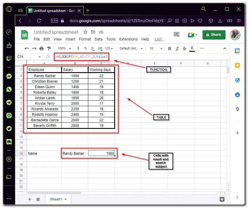
As you can see everything is quite simple. It doesn’t take much time to search for numbers in the table this way. The function is easy to understand and very easy to create. The main thing is to enter the correct search sub-item because the function will search for exactly what you have entered.
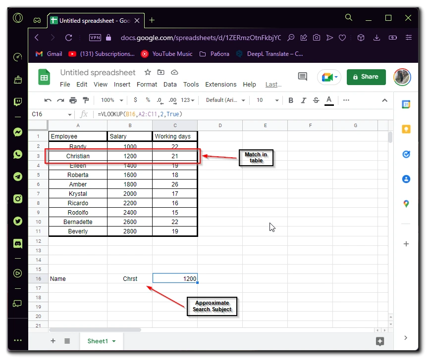
How to use VLOOKUP in Google Sheets with an Approximate match
A slightly different case would be when you want to find something but don’t know the exact Search Subject. In this case, you can change the function to search for approximate results that are as close to the Search Subject as possible. In this case, the function will look like this
=VLOOKUP(B16;A2:C11;2;True)
As you see, only the last parameter was changed, when you set TRUE at the last parameter, the function automatically selects all variants which are closest to your Search Subject. In the example it looks like this:
Also, an interesting feature for you might be the ability to import one table to another. If you combine this with the Search function, you can very quickly process many different tables.
Read also:
- How to fix formula parse error in Google Sheets
- How to count non-empty cells in Google Sheets
- How to use the ARRAYFORMULA function in Google Sheets
How to import data to another Google Sheet
A very handy feature in Google Sheets is importing tables from other files. All you need to do is to have them in your account and you have editor access to them. For example, you can create yourself a Master Sheets and from it already import data into different tables, for example for your employees. To do this you need to:
- Select the cell where you want to import the data and start the function with “=IMPORTRANGE“.
- Then you have to enter a link to the table you want to import.
- At the end, specify the name or the column range of the table you want to enter.
- The resulting formula would look like this:
=IMPORTRANGE("your_link";"sheet1!A1:C10")
After that, the data from the original table will be automatically imported. To change the data in this table, all you have to do now is make edits to the original table and they will automatically be pulled into the new table. Be careful and keep your tables in order so that you can manage them comfortably and they don’t just turn into a pile of numbers.


