Google Sheets is a handy tool universally used by companies working in the digital sphere. With its help, it’s convenient to plan (for example, content, finances, or tasks), do accounting, conduct marketing analysis, make forecasts, etc. You can work with spreadsheets in a web browser or apps for smartphones and tablets.

Google Sheets is a multifaceted and functional tool with many possibilities and use cases. This service contains a bunch of formulas you could write a book about. Google tries to make its services as easy to use as possible. That’s why they’ve added such a great feature as ARRAYFORMULA. It allows you to stop copying formulas into every cell all the time and simplifies a lot of processes. Well, here’s how to use the ARRAYFORMULA function in Google Sheets.

How does ARRAYFORMULA work?

Before you use this function, you need to understand how it works and what it consists of. Well, as the name implies, this is a formula for an array. An array is a range of cells arranged in rows and columns. And the formula is a special command that performs an action or calculation on the specified cells.

So you can conclude that an array formula allows you to perform several calculations on a group of cells at the same time. With an array formula, you can get one or more results depending on the calculations being performed. You can use an array formula to get one or more results, depending on the calculations you perform. For example, you can create a Gantt chart in Google Sheets and make changes to it using ARRAYFORMULA for multiple cells.

The ARRAYFORMULA function displays values from an array formula in multiple rows and columns. It also allows you to use arrays in some functions, extending their capabilities. It’s of main interest in tasks of array processing, avoiding errors when copying formulas of the same type, and creating arrays from ranges. Many array formulas are automatically expanded to neighboring cells to avoid explicit use of the ARRAYFORMULA function.

Read Also:

• How to hide tabs from specific people in Google Sheets
• How to create a master sheet in Google Sheets
• How to turn on dark mode in Google Sheets

How to use ARRAYFORMULA in Google Sheets

The syntax of the ARRAYFORMULA function is quite simple. The function requires only one argument. The argument can be a range of cells, an expression, or a function for one or more arrays of the same size.

There are a total of two ways to insert an ARRAYFORMULA formula into Google Sheets. The first way is good if you have already typed the formula and you understand that you want to use the ARRAYFORMULA function.

• When you enter a regular formula in a cell, place your cursor on the formula or the formula bar.
• Then press “Ctrl + Shift + Enter” on Windows or “Command + Shift + Return” on Mac. You’ll see your formula turn into an ARRAYFORMULA formula.
• Just press “Enter” or “Return” to apply the transformed formula.

Another way to insert an ARRAYFORMULA formula into Google Sheets is to enter it like any other formula. Moreover, you can also insert this formula in the hidden cells in Google Sheets.

What is the example of the ARRAYFORNULA?

Let’s do a simple multiplication calculation for a range of cells as an example. Let’s take the number of items sold and multiply it by the price per unit. To do this for the whole array, you need to use the following formula:

• =ARRAYFORMULA(B2:B5*C2:C5)

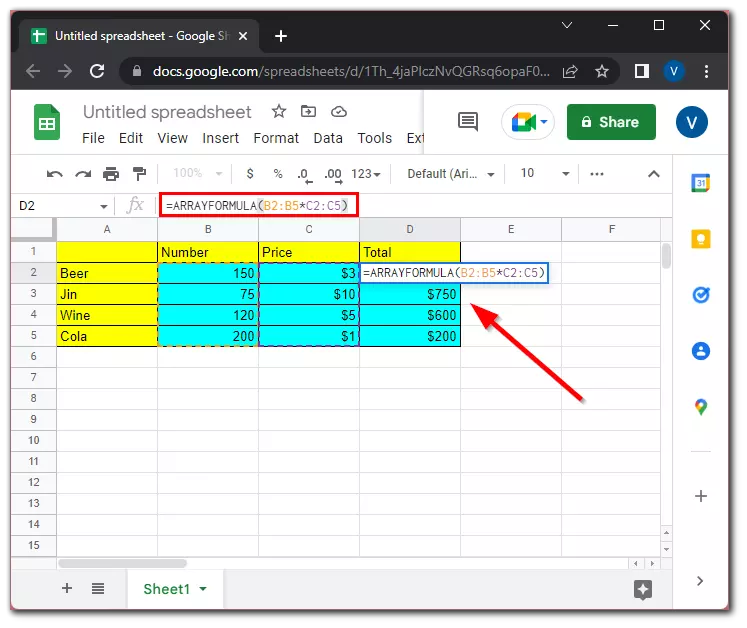
As you can see on the screenshot, using this formula, you can calculate the arrays of all the cells you specify at once. This is very useful if you need to keep a permanent record of how much was bought or sold goods or other services.

Google Sheets instantly calculated everything and fill in the appropriate cells with the correct data. Of course, sometimes there are certain errors in the calculations. However, this is often mostly due to human error rather than system error. For example, if you encounter a formula parse error in Google Sheets, you have to be aware that you can easily fix it. Just check your formula and enter the right command.

What can be done with rows, columns, and cells in Google Sheets?

Cells, columns, and rows are the main entities in Google Sheets. You can perform various actions with them:

• Add new ones. To do this, select a cell, row, or column, right-click and select the desired item in the list. Rows can be added above and below, columns – to the right and left, and cells – shifted to the right and down.
• Delete the contents of cells and the cells themselves, as well as columns and rows. To delete contents, select the desired cell or range and press “Delete” or “Backspace”.
• Move filled columns, rows, and cells. The easiest way is to select the desired element, place the cursor on the edge so that it turns into a hand, press the left mouse button, and drag it to the desired location.
• Group columns and rows. Useful when you want to “hide” several elements so they don’t get distracted.
• View the history of changes. This is a relatively new tool in Google Spreadsheets. In addition to the standard version history for Google services, you can now see what has been changed in a particular cell in tables.
• Convert to a user card. Another new feature. You can add the card of any person you’ve communicated with via email in Gmail to a cell. When you hover your mouse over it, a panel pops up from which you can view information about the user, add them to your contacts, send an email, start a video meeting with them, or create an event.
• Combine columns, rows, and cells. This is often necessary when creating tables that are complex in structure. To merge, select the desired elements and click the appropriate icon on the toolbar.

Furthermore, you can also make the columns to be the same size in Google Sheets.

Read Also:

• How to insert check mark in Google Sheets
• How to set the print area in Google Sheets
• How to use the slicer in Google Sheets

What data formats are available in Google Sheets?

For the convenience of data management, different formats are used, which are displayed differently in tables. There are dozens of options available in the service, but the most commonly used are:

• text
• numeric
• financial
• currency
• percentage
• time
• date

Only numeric data is used for analytics, such as finding correlations or averages. To change the view, use the “Format” section and select the desired settings. If the general menu doesn’t have what you need for the layout, click the “Other formats” tab – there’s a complete list.